Block Averaging and Bootstrapping: Estimating the mean from autocorrelated data

Why hello, lovely readers!

Today I’m going to pick up where I left off last week: estimating the mean from correlated data. Last week I discussed how a traditional statistician might go about calculating the average and its error bars; we saw where it works well (random data) and where it works poorly (data correlated with its own history).

This is an important topic in statistical mechanics (the field where I currently work). I run computer simulations of molecules (DNA!) and calculate many different values from those simulations. One such value might be the distance between hydrogen atom A and carbon atom B. You can imagine that this distance doesn’t just randomly jump about- it is strongly influenced by where it’s been. It’s not enough to know the average distance, it’s also important to know how accurate that estimation is… the crux of our problem.

Today I’m going to explore two possible approaches to solving our error-estimation difficulties: block averaging and bootstrapping. We’ll go over what each one is, how well they each work, and the shortcomings of each approach. We’ll wrap up with a preview of next week’s work which leaves the Frequentist domain and enters the world of Bayesian statistics. (Don’t be alarmed if you don’t know what that means, that’s what next week’s post is all about!)

Alrighty then! Let’s dive into…

Block averaging

Wassat?

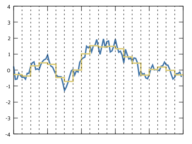
Recall our data from last week:

If we take a data point at time t, a certain time after t, we can safely assume that our data is uncorrelated. Imagine if you were walking down the street and tripped on a crack:1Don’t worry, no one saw you. for several steps after you would have very irregular footfalls- they would be longer than usual and have highly uneven spacing between them. After two to five steps, when you have recovered, the correlation between your current footfalls and the step you took when you tripped is barely even noticeable. A block down the road and you probably can’t tell the difference.

We’re using the same idea here. Let’s divide our data up into chunks (or, dare I say… BLOCKS!) and look at the trends between the average of each block:

If the blocks get large enough, they should be uncorrelated from each other. That means we can treat each block as an individual data point and calculate the average and standard deviation from that.

But what size should the blocks be?

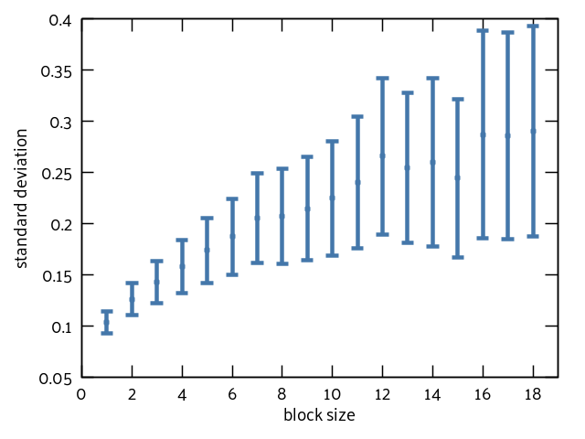
Ah, the million dollar question. Too small and you still have autocorrelation. Too large and your error bars go off to infinity. Ideally we want to find the smallest block size that will give us uncorrelated data. After the data is uncorrelated, increasing the block size should give us the same standard deviation over and over again (assuming a normally distributed sample). So we’re looking for the point at which the standard deviation “levels off” with increasing block size.

Here’s the plot for my data:

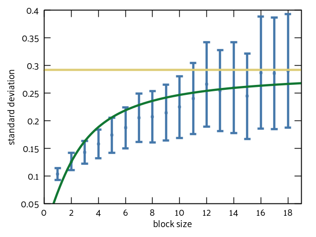
Eyeballing this, it looks like the data levels off at ~0.25 or ~0.3. It’s a little tricky to tell because my sample only has 100 data points. I read through a lot of literature to see if there was a definitive way to choose the ideal block size. I didn’t find much. Clarification: I didn’t find anything. I decided to fit my data to the function y = a * arctan(b*x) because that seemed like the closest shape to what we’re trying to predict. At that point I calculated the value of the asymptote (where everything “levels off”) and used that for my value of the standard deviation:

It’s an okay fit. It’s also an okay approximation: I generated 1000 sets of autocorrelated data and asked my program to find the mean (and error bars) with a 95% confidence interval. Remember: this means that if everything goes according to plan, 950 of those sets will contain the actual mean in the calculated range. I got 672. Not the 950 we’re looking for, but still better than the 124 from the “naive” method explored last week.

Can we do better? Let’s try…

Bootstrapping!

To be fully honest, I went into this not really sure if bootstrapping would be a good idea or not. I wanted to write some bootstrapping code, and I wanted some toy data to play with while I did it. Bootstrapping can be very powerful for projects like machine learning and data validation, but is it for mean-estimation? No, no it is not. I got data almost as bad as for the naive approach.

Why am I still writing about this, then? Well, I think it’s A) useful to understand what bootstrapping is, B) useful to understand what it is not2And it IS NOT a tool for this particular puzzle, and C) useful to see what others have done, even if that is a negative result.

So… What is bootstrapping?

Bootstrapping is a resampling method. In machine learning (or other data science fields), you often have “training data” that you want to train an algorithm on. Maybe you want to predict the price of a house, or guess which movie a particular use might like to see. You need to give your computational model some input that it can learn from.

You also need some data you can test the model on. It is commonly taught3read: was taught in my machine learning class that you segregate a portion of your data as a “validation set”; you don’t train on this data, you instead use it to check your model. Bootstrapping takes a different approach. It uses ALL of the data for training and ALL of the data for validation.

A reasonable human4or reasonable AI overlord might ask how that is statistically sound. That is a very reasonable question, reasonable human5and/or overlord! Bootstrapping creates thousands of validation sets by randomly sampling from all of its data. Each validation set is the same size as the original data, and data points are allowed to repeat. That’s called sampling with replacement. If all of the validation sets check out, that’s great! It means your model works on all of the data aggregated (because you trained it to) but also that it works on multiple random subsets of your data (not just one).

Why doesn’t it work for this project?

Well, a lot of reasons. I put on my thinking hat for this one. I had originally thought that randomly sampling from the data would overcome the auto-correlation, but after doing my best Pooh Bear impression6think think think I realized that the correlation is still in there.

Block averaging takes a structured approach to removing the correlation that is time-dependent. It blocks all of the correlated data together so it can be removed. Bootstrapping is random. It can’t de-correlate the data because it ignores any of the historical/time context that the data occurs in.

I also came to realize that this is just straight up the wrong kind of problem to use bootstrapping on. Bootstrapping is for validating an already existing model. It is not for making the models in the first place. While it seems like finding the error in a mean could be considered “validating,” it turns out that my model IS that error. I’m trying to predict the error in my mean. I could use bootstrapping to check the errors I calculate, but given that I can basically generate new data for free… eh. It’s not that useful.

But how did it do?

Of the 1000 data sets that I fed it, my bootstrapped algorithm (aiming for a confidence interval of 95%) correctly included the actual mean… 233 times. It was supposed to capture the real mean 95% of the time and it got… 23%. Ouch.

A parting thought on bootstrapping

While this did give me crappy results for the autocorrelated data, it was a really good predictor for completely uncorrelated data. That makes sense, because the uncorrelated data can actually benefit from random sampling. It’s already normally distributed (because of how I generated it), so choosing from it randomly should give a normal distribution. Bootstrapping helped even out some of the noise in this instance. I don’t know if that’s useful for anything, but hey, it does illustrate well what bootstrapping DOES do well.

So what about this Bayes stuff you mentioned earlier?

I’m all about that Bayes.7I’m sorry. I had to.

Everything I’ve discussed this week and last has been Frequentist statistics. These are the methods I learned in college. Heck, these are the methods I’ve learned in graduate school. I hadn’t heard of Bayesian statistics until halfway through my PhD.8Assuming I graduate next August, which is the plan. Researchers love Bayes! But why? What is this mystical brand of statistics? Bayesian proponents think of it as a way to solve basically every statistics puzzle. Can it solve this one?

Tune in next week to find out!!